This post is an intro to DSE Graph with a focus on the strategies that should be used to load large graphs with billions of vertices and edges. For those familiar with DSE Graph and large graph strategies or those who want to dive directly into loading data, proceed to the next post in this two part series entitiled Large Graph Loading Best Practices: Tactics.
Intro to DSE Graph
DSE Graph is differentiated from other graph databases by building on DataStax Enterprise's scalability, replication, and fault tolerance.
Note - To understand how DSE Graph data is stored in DSE's Apache Cassandra(TM) storage engine, check out Matthias and Marko's posts on the matter.
When folks ask me where DSE Graph falls in the greater database / graph database landscape, I use this image to communicate the combination of scalability and value in relationships that make DSE Graph such a unique product:
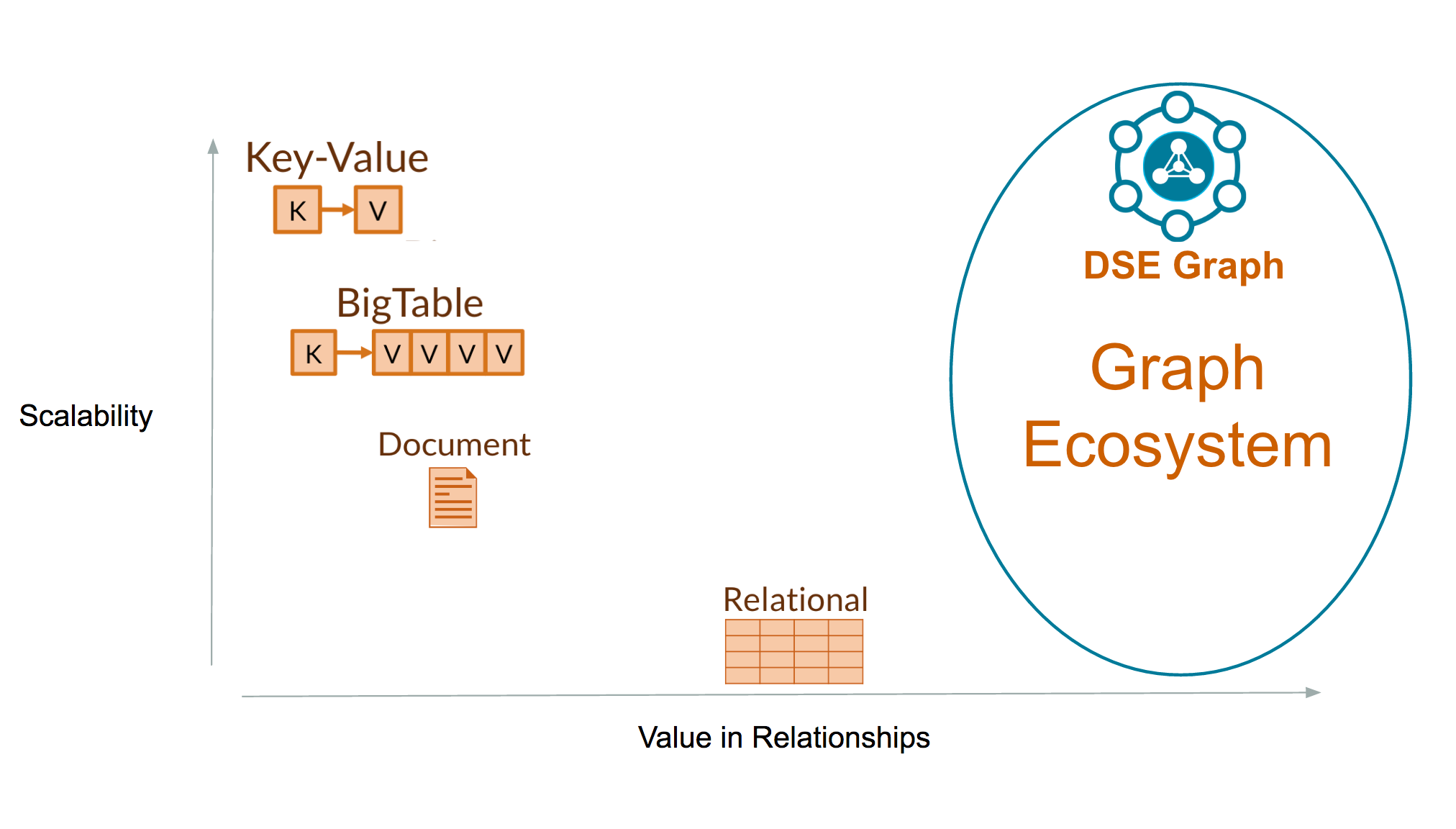
DSE Graph is positioned on the right side of the chart where relationships are most valuable, and toward the top of the chart due to the scalability it inherits from DSE and Cassandra. The third key aspect that differentiates DSE graph is the velocity of the data it can support. Unlike analytical graph engines which load a static graph to memory and then crunch that static graph for insights, an operational graph is constantly changing as the real world concepts whose relationships and vertices it represents are created, updated, and deleted.
Key Takeaway - DSE Graph is designed as a real-time, operational, distributed graph database.
Motivation and Goals: Playing with Scalable Graphs
If you have distributed graph problem, you may want to bulk load your data into DSE graph and start querying. However, loading significant amounts of data (>1 billion V's or E's) into graph dbs is a time consuming, nontrivial task. The purpose of this article is to summarize some key design considerations related to dealing with large graphs.
Large graphs, idempotence, and scalability
Idempotence is a common concept in distributed systems design. If an operation is idempotent, it can be repeated over and over and still yield the same result. We use idempotence to help us solve problems like the fact that exactly once delivery does not exist, it also greatly simplifies the design of our systems, minimizing bugs and promoting maintainablility. For the purposes of two part article series, we are going to focus on building scalable distributed idempotent graphs. This is one of the design choices that is supported in DSE Graph but note that not all graphs that can be built on DSE graph will have idempotent vertices and idempotent edges.
Idempotent Vertices
DSE graph allows two types of vertices, 1) those with system generated keys and 2) those with custom ids. For the purposes of this two part series we are going to concentrate on custom ids. Custom ids are useful for large graph problems in that they allow developers to take graph partitioning into their own hands. Custom ids will feel familiar if you have used DSE or cassandra and understand data modeling.
You configure the partition key of your Vertex label with a DDL operation:
schema().vertexLabel('MachineSensor').partitionKey('manufacturing_plant_id').clusteringKey('sensor_id').create()
If you are using custom ids, the partition key is required and the clustering key is optional. For more on Cassandra data modeling and clustering keys vs. partition keys see my post on data modeling for DSE.
Note - your partition key, clustering key combination should provide uniqueness for the vertex. With this configuration, reinserting will not generate duplicates
Idempotent Edges
DSE Graph edges support different cardinality options. For multiple cardinality edges (where there can be more than one edge between the same two vertices of the same edge label type) edge creation is not idempotent.
For the purposes of this two part article series, we will focus on single cardinality (thereby idempotent) edges. You can create single cardinality edge lables in DSE Graph use the single() keyword:
schema.edgeLabel('has_sensor').single().create()
Let's load!
Having considered the strategies mentioned above, let's proceed to the second part which adresses the tactical aspects of loading large graphs.